www.bcb.lon.ac.uk
Summary
Data Pre-Processing
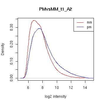
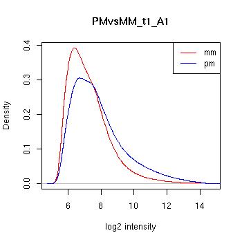
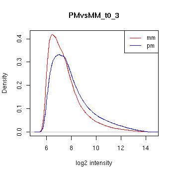
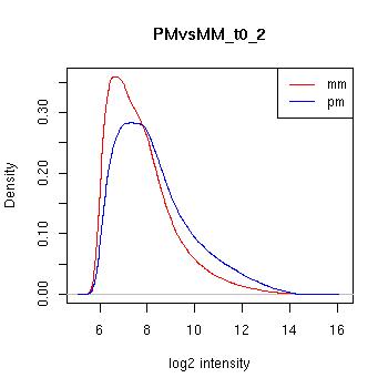
Quality Control Plots:
Boxplots
Reproducibility between replicates
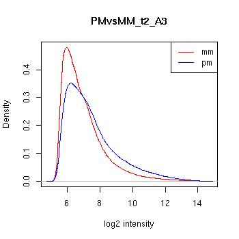
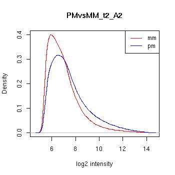
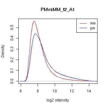
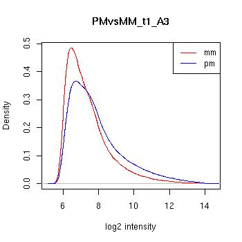
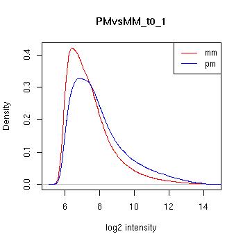
PMvsMM Histograms
RNA Degradation
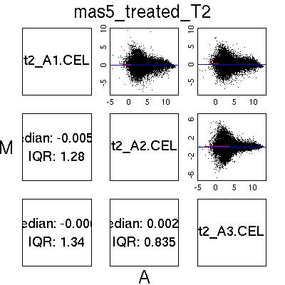
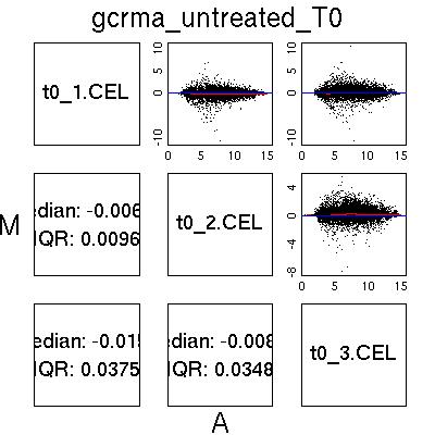
MvA Plots
Control Probeset Analysis
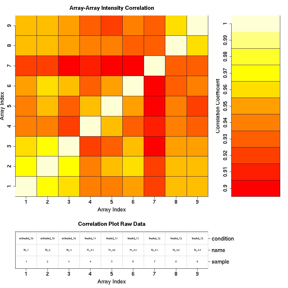
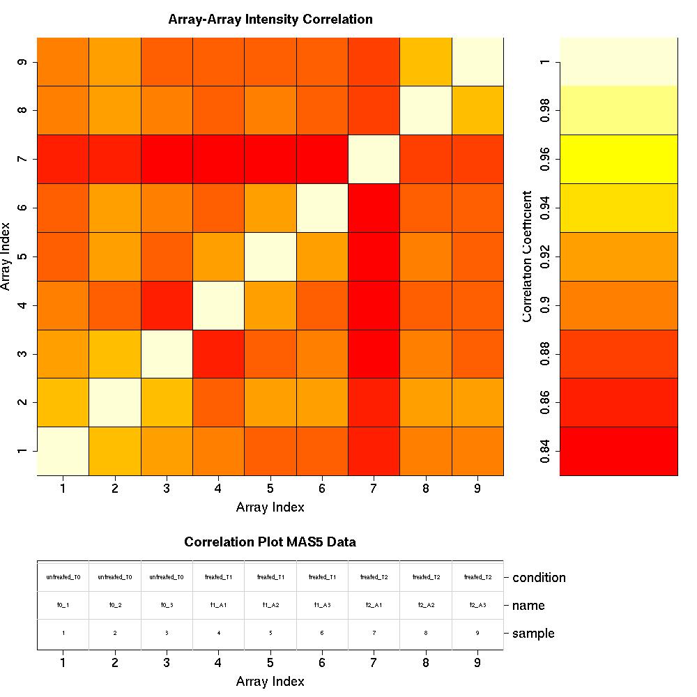
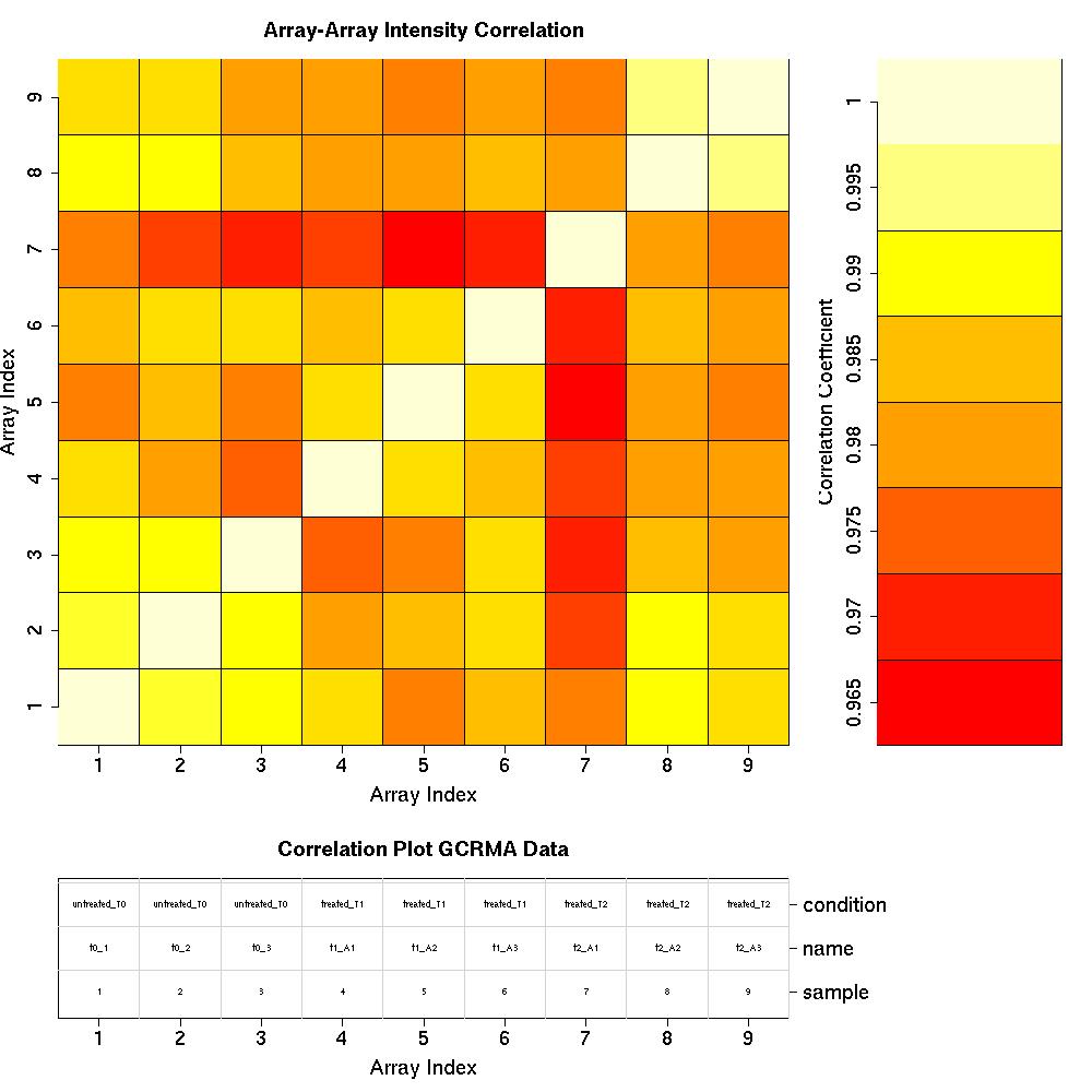
Correlation Plots
Appendix
| Customer: | | Joe Blogg |
| | | Joe.blogg email |
| Author: | | Sonia Shah |
| | | |
| Chip Type: | | HU133A |
| Summary: | | The GeneChip data comprising this experiment pass the QC criteria with no warning flags. |
File descriptions:
| array index | file | condition |
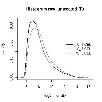
| 1 | t0_1.CEL | t0_1 |
| 2 | t0_2.CEL | t0_2 |
| 3 | t0_3.CEL | t0_3 |
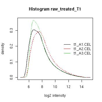
| 4 | t1_A1.CEL | t1_A1 |
| 5 | t1_A2.CEL | t1_A2 |
| 6 | t1_A3.CEL | t1_A3 |
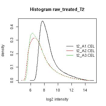
| 7 | t2_A1.CEL | t2_A1 |
| 8 | t2_A2.CEL | t2_A2 |
| 9 | t2_A3.CEL | t2_A3 |
The experiment is looking at the effect of compound A on gene
expression. Samples were collected at three time points: 0hr (t0 - no
compound treatment), 1hr after treatment (t1) and 2hrs after treatment
(t2). The experiment was done using 3 biological replicates for each
time point.
Top
Pre-processing of Affymetrix data involves three
steps: background adjustment, normalisation and summarisation.
Normalisation adjusts the data to make the measurements from different
arrays comparable. Summarisation combines the multiple probe
intensities for each probeset to produce a single expression value for
each probe set. We use the following two methods:
- MAS5.0 corrects for hybridisation to the
mismatch (MM) probes for that particular probeset. The output is an
expression value which we convert to log2 prior to further analysis. We
do not filter on Absent, Present, Marginal calls. We then perform a
between-chip loess normalisation on all GeneChips included in the
experiment. The intensity values (log2) for the MAS5-normalised data
can be found in file MAS5_loess_log2.tsv, which can be opened in Excel
(.tsv is tab-separated value).
- GCRMA is an alternative method which
calculates a background adjustment step that ignores the MM intensities
(RMA; Robust Multi-Array Analysis), which also incorporates sequence
information from the probes (GC). This method performs within-chip and
between-chip normalisations in a single step. The intensity values
(log2) for the GCRMA-normalised data can be found in file GCRMA.tsv,
which can be opened in Excel.
Other normalisation methods available are Plier (Affymetrix), Li Wong (dChip) and RMA (no GC correction).
Top
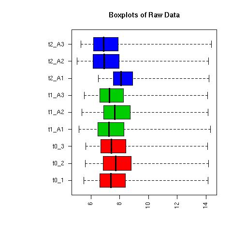
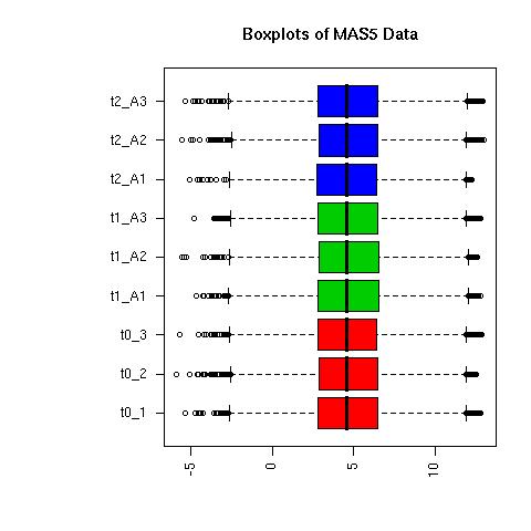
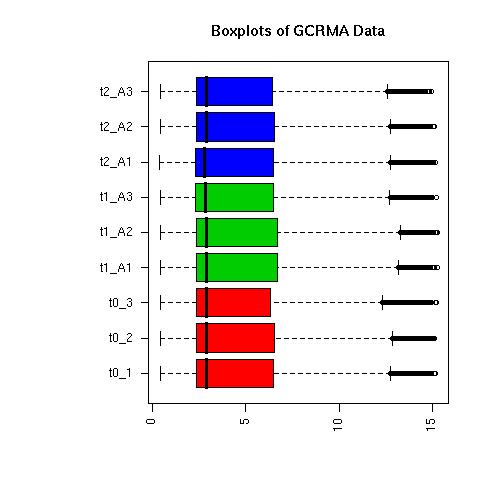
QC Plots
| Pre-normalised Data |
 |
| Normalised Data |
 |
 |
Top
Pre-normalised Data
MAS5 Normalised Data
GCRMA Normalised Data
Top
Top
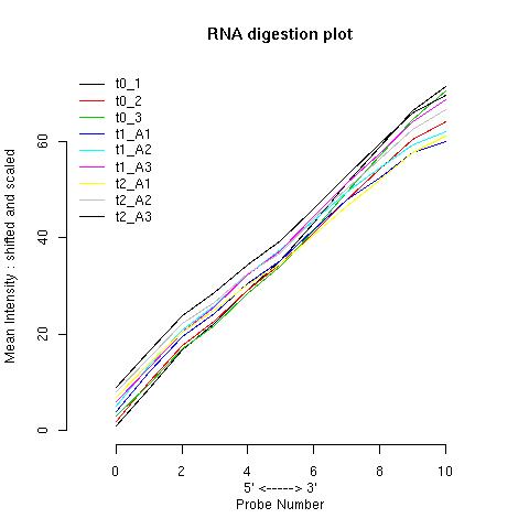 |
| chip | slope | p-value | | t0_1 | 7.09 | 3.05e-14 | | t0_2 | 6.22 | 4.74e-13 | | t0_3 | 6.77 | 3.66e-13 | | t1_A1 | 5.62 | 7.2e-11 | | t1_A2 | 5.7 | 9.7e-11 | | t1_A3 | 6.3 | 1.24e-14 | | t2_A1 | 5.39 | 3.93e-13 | | t2_A2 | 5.85 | 1.32e-13 | | t2_A3 | 6.07 | 2.4e-13 |
|
Top
Click on the plots for a larger image
Top
Top
Click on the plots for a larger image
Top
References
The data was analysed using Bioconductor v1.5 and R version 2.1.0
Bioconductor: open software development for computational biology and bioinformatics
Wu et al., GCRMA normalisation
Miller et al. Simpleaffy package
TIGR MeV v3.1
Affect of RNA Amplification on RNA Degradation
Higher degradation is to be expected when an extra round of RNA
amplification has been used, so reference chips must be chosen
carefully.
To illustrate this, the RNA degradation plot below was made using
published data from several mouse M403_2 chips. These datasets were
downloaded from the Gene Expression Omnibus,
GEO. The comparison used data obtained from eight chips hybridised with Universal Mouse Reference RNA Samples from Stratagene.
n
| GEO Sample ID | RNA Sample |
| GSM24056, GSM24057, GSM24058 | MUR OneRNA |
| GSM24060, GSM24061 | MUR TwoRNA |
| GSM24062, GSM24063 ,GSM24064 | MUR RS 10ng-1 |
OneRA: One round of amplification
TwoRA: Two rounds of amplification
RS   : Ribo-SPIA amplification
| Samples | GSM24056-GSM24058;
GSM24060-GSM24061;
GSM24062-GSM24064
|
| Slope | 1.07, 1.03, 1.05,
5.35, 5.24,
4.51, 4.58, 4.48
|
| Pvalue | 3.98e-04, 7.90e-04, 5.86e-04,
1.02e-12, 4.90e-13,
1.03e-10, 9.54e-11, 8.43e-11
|
| 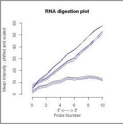 |
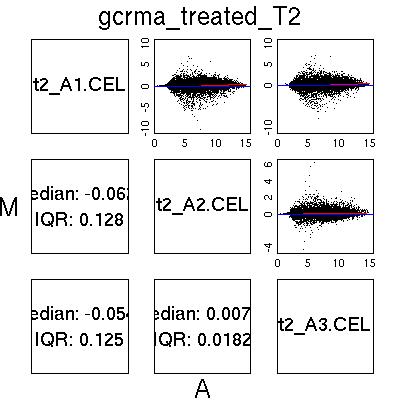
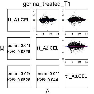
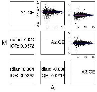
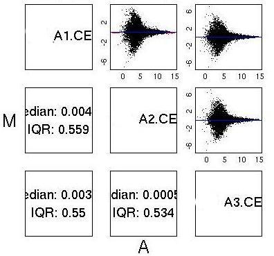
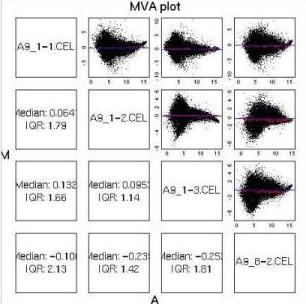
MvA Plots
| Type of Samples and Comments | MvA Plots |
| GCRMA normalised data from two ‘good’ chips. Notice the almost
flat Loess line (red) and the near symmetric nature of the plot about
the A axis.
|  |
| MAS5.0 and Loess normalised data from two good chips. Once
again the plot is almost symmetric about the A axis, although notice
the different shape to the plot, with larger peaks around A=4. This is
characteristic of MAS5.0 normalised data and not a QC issue. |
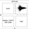 |
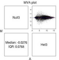
| MAS5.0 normalisation on an extremely poor set of 4 chips.
Notice that although there is still some of the characteristic MAS5.0
shape to the plots, the loess lines in red are not particularly
straight. None of the plots is remotely symmetric about the A axis:
each of the plots shows a distinct skew for higher A values. |
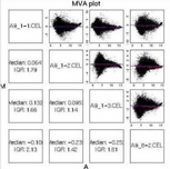 |
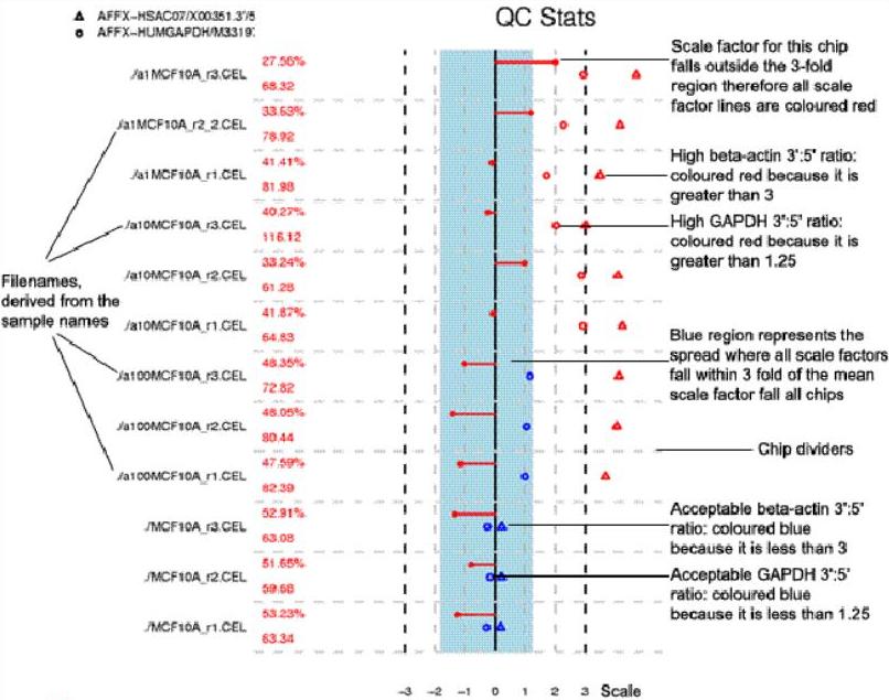
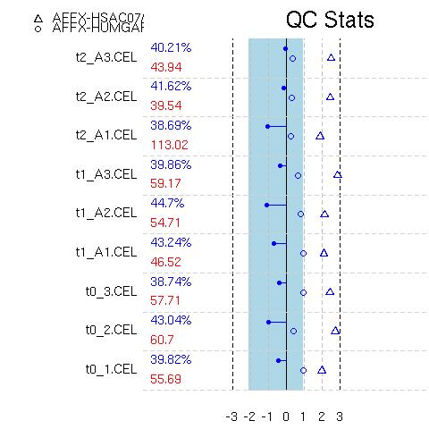
SimpleAffy QC
A number of additional QC assessments can be made on the MAS5.0
normalised data using the BioConductor library Simpleaffy. These are as
follows:
- Average background
This should be similar across all chips.
Differences could be due to unequal amounts of RNA in the hybridisation
step or due to one of the hybridisations incorporating more label, thus
producing a ‘brighter’ chip. Values are given next to each chip,
underneath the %Present call.
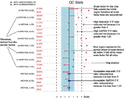
- Scale factor
MAS5.0 scales the intensity for each sample so that each array has the
same mean; the amount of scaling required is given by the scale factor.
A broad range of scale factors across the arrays would indicate
differing amounts or quality of RNA. Affymetrix recommend that scale
factors should lie within 3-fold of each other. The blue stripe
represents this range of acceptable scale factors.
Scale factors are plotted as dots on the end a line from the centre of
the image. A line to the left indicates down-scaling; a line to right
indicates up-scaling. Were any of the scale factors to fall outside the
strip, they would all be coloured red.
- Number of genes called ‘Present’
By generating Present/Marginal/Absent calls, the fraction of genes
called ‘Present’ (‰Present) can be calculated for each array. As
before, differing amounts or quality of RNA can lead to a broad range
of %Present values across the arrays. Variation between different
tissue types or samples may be expected. However, the %Present values
of replicates ought to be similar. Values are given to the right of
each chip name, on the left hand side of the plot.
- 3’ to 5’ ratios
3’ to 5’ ratios provide a measure of the quality of the RNA used.
Rather than the previous RNA degradation graphs which considered all
probes across an array, Simpleaffy looks specifically at Β-actin and
GAPDH, two relatively long genes. The reasoning is similar: by
comparing the intensity values from the 3’ probeset to the 5’ or
mid-point probesets a 3’:5’ ratio can be calculated. A high ratio
indicates significant RNA degradation or a poor in vitro transcription
(IVT) step.
GAPDH 3’:5’ ratios are plotted as circles – ratios > 1 are coloured
red (unacceptable). Β-actin 3’:5’ ratios are plotted as triangles.
Being longer than GAPDH, unacceptable ratios are > 3 and also
coloured red. Acceptable ratios for both are coloured blue.
- Spike-in probesets
Additional labelled cRNAs are added to validate the hybridisation step.
BioB is added at a concentration of 1.5pM. This amounts to roughly 3
transcripts per cell which is the lower limit of detection for the
Affymetrix system. Ideally BioB should be called ‘Present’ on every
array, but a lower bound of 70% Present across all arrays is considered
acceptable. This information is not plotted but can be obtained using
the R command outlined above.
An example SimpleAffy QC plot is shown below. More information on these QC metrics can be found in the SimpleAffy website from which this plot was taken.