www.bcb.lon.ac.uk

Microarray Data Analysis Sample Report

Summary

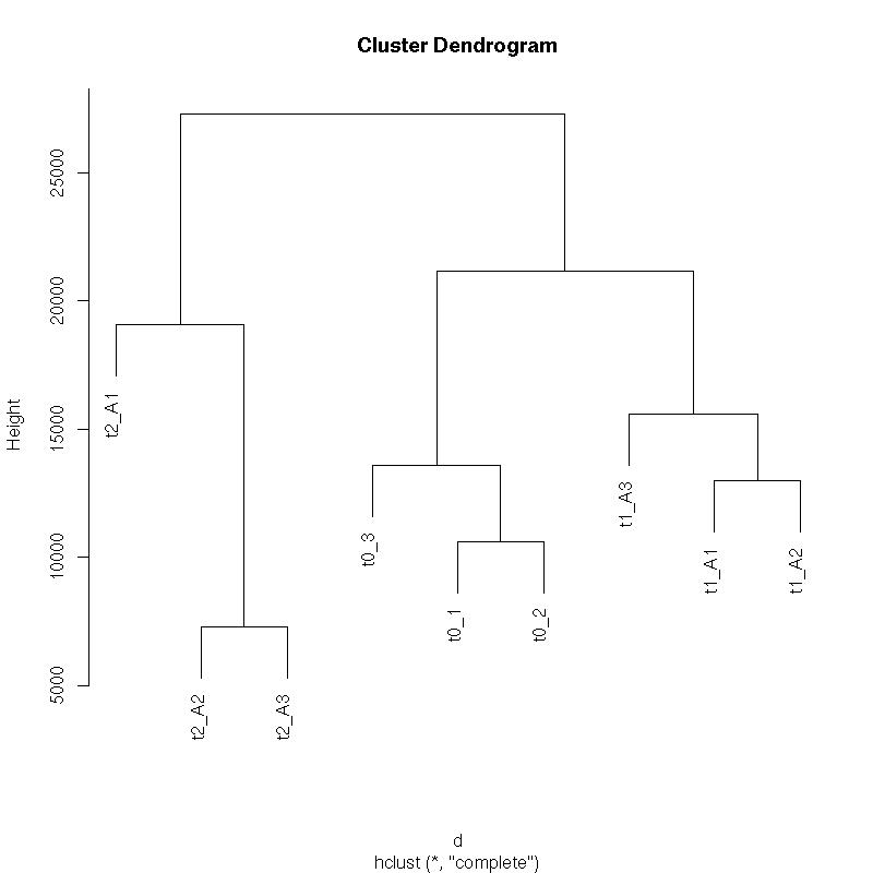
Sample Clustering

Differential Expression using Limma
   Volcano Plots
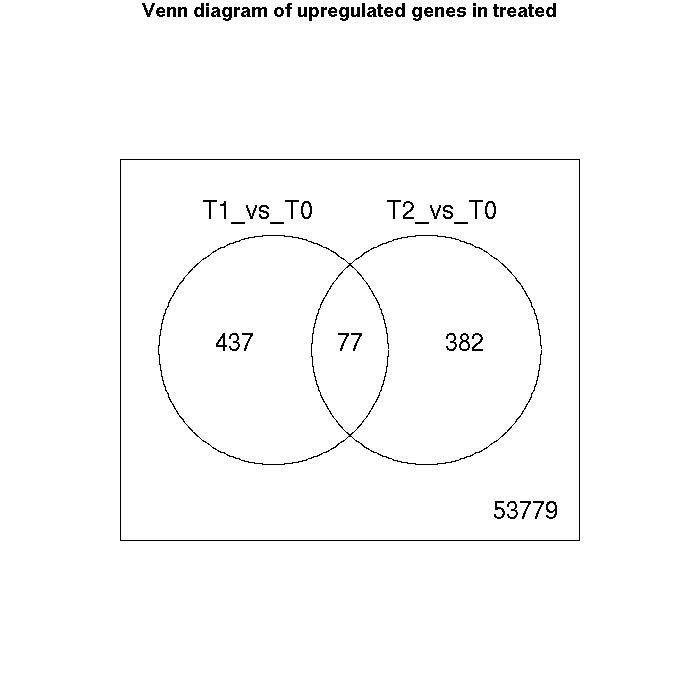
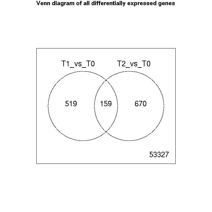
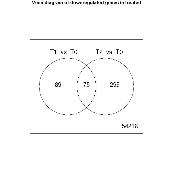
   Venn Diagrams

Appendix

Report Summary

Sample Clustering

The gcrma-normalised data were clustered on samples using the Manhattan distance metric, with average linkage. Data from the same sample groups (biological reps) should cluster together.

Comment:

All biological replicates cluster together. As expected, the first time point T1 has expression that is more similar to time 0 (T0) than the T2 later time point

Differential Expression using Limma

A simple approach to looking at differential gene expression between conditions is to select genes using a fold change criterion. This may be the only option when very few or no replicates are available. Such analysis does not allow for the assessment of significance of expression differences in the presence of biological and experimental variation, which may differ from gene to gene (Gentleman et al). Therefore, where possible statistical tests should be applied to assess differential expression.

In most cases the statistical test is applied to an entire dataset rather than a single gene. In essence, you are testing many hypotheses simultaneously (multiple hypothesis testing). This potentially results in a large number of falsely significant results. Therefore we must also correct for multiple testing. There are several methods that can be used. We use the Benjamini-Hochberg (FDR) test for multiple correction and use a p-value cut-off of 0.05. This means that all genes that have an fdr-adjusted value of less than 0.05 are considered as differentially expressed and the expected proportion of false discoveries is controlled to be less than 5%.

All conditions were compared with each other resulting in 10 contrasts or paired t-tests. The t-tests were performed on GCRMA-normalised data. The results for each comparison are shown in the summary tables below, which show the number of genes that are up-regulated, down-regulated or show no change between the two conditions being compared.

Comment:

The lists of significant genes for each comparison have been saved as excel files.

Links to external databases for all the differentially expressed genes can be found in the T1_vs_T0.html and T2_vs_T0.html files.

Volcano Plots

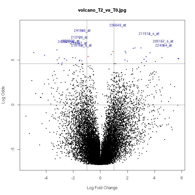
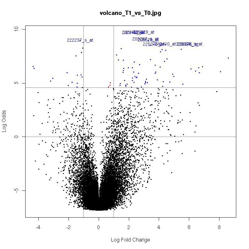
plot of log-fold changes versus log-odds of differential expression.

The Log Odds (or B value) on the y-axis is the odds (or probability) that the gene is differentially expressed. A Log Odds value of 0 (horizontal line in each graph) corresponds to a 50-50 chance that the gene is differentially expressed. The higher the Log Odds for each gene, the higher the probability that the gene is differentially expressed and not a false positive.

The x-axis indicates the log2 value of fold-change between the two conditions.

Each gene is represented on the plot as a single dot. The blue dots are genes that have a log-odds value equal to or more than 4.6 (99% probability that the gene is differentially expressed between the the conditions being compared) and also show a fold change of 2 or more between the two conditions being compared. The red dots are genes that although have a log odds score of 4.6 or more, have a fold change less than 2-fold. The top ten most significantly differentially expressed genes are labelled with their probe ID.

Genes which are significantly up-regulated in the first treatment compared to the second treatment are located in the upper right square of each graph (these have a positive log fold value).

Genes which are significantly down-regulated in the first treatment compared to the second treatment are located in the upper left square of each graph (these have a negative log fold value).

Genes in the lower left and right squares of the graph are probably false positives.

Click on the images for a larger image

Comment:

Venn Diagram

Comment:

Appendix

The data was analysed using Bioconductor v1.5 and R version 2.1.0

Bioconductor: open software development for computational biology and bioinformatics

Wu et al., GCRMA normalisation

Miller et al. Simpleaffy package

TIGR MeV v3.1

Gentleman et al. Bioinformatics and Computational Biology Solutions Using R and Bioconductor. Springer, 2005

Linear Models (limma) Statistics

The Linear Models package uses Bayesian statistics to compute the probability of a gene being differentially expressed in any defined contrast. Bayesian statistics is a means of measuring the probability of an outcome (i.e. a gene being differentially expressed), calculated from a ratio of the probabilities of the experiment outcome and the prior assumption of the experiment outcome (the null hypothesis - nothing is differentially regulated).

The summary statistics are computed for each gene and each contrast (i.e. experiment comparison such as treated vs. control). These include:

M-value(M) - log2 fold change for that gene. A positive value indicates up-regulation of a gene, a negative value indicates down-regulation.

A-value(A) - average expression value for that gene across all the arrays

t - moderated t-statistic is the ratio of the M-value to its standard error. This has the same interpretation as the ordinary t.statistic except that the standard errors have been moderated across genes, effectively borrowing information from the ensemble of genes to aid with inference about each individual gene.

p-value - obtained from the distribution of the moderated t-statistic, usually after some form of adjustment for multiple testing such as Bonferroni or Benjamini-Hochberg.

B-statistic (B or lods or Log Odds) - is the log odds that the gene is differentially expressed. A B-statistic of zero corresponds to a 50-50 chance that the gene is differentially expressed. That is, a B-value of zero means the probability of the gene being differentially expressed (the outcome of the experiment) is equal to the probability that it is not differentially expressed (null hypothesis).

Example : A gene has a B-value of 1.5. The odds of differential expression is exp(1.5)=4.48, or about 4.5 to 1. The probability that the gene is differentially expressed is 4.48/(1+4.48)=0.82 or 82%
B-value = 0.3, odds = 1.35 to 1, probability = 57%
B-value = 4.6, odds = 99 to 1, probability = 99%

The B-value and the moderated t-statistic rank the genes in the same order (given that there are no missing values in the data). p-values and B-values also usually rank the genes in the same order. All three measures are closely related. A low p-value, and a high B-value should indicate the ranking (i.e. most significant=1 to least significant=54675 (or number of genes on array)) in the dataset for that particular contrast. The ranking will vary for each gene depending on the comparisons made between samples.

Multiple Correction

The most common form of multiple testing is "fdr" which is Benjamini & Hochberg's method to control the false discovery rate. If all genes that have an fdr-adjusted value of less than the threshold, let say 0.05, are considered as differentially expressed then the expected proportion of false discoveries is controlled to be less than the threshold value, in this case 5%.

In another method, the Bonferroni correction, the chance of making even a single type I error (false positive) can be maintained at the desired level, which in this case 5%. Bonferroni is more stringent than the Benjamini-Hochberg method.

Annotation of probesets

Probeset annotation is derived from the NetAffx site (www.affymetrix.com, free access but login required). Please note that while the NetAffx annotation is revised regularly we recommend that the annotation is confirmed before further experiments such as qPCR. This can be done by Blasting the probe or probe target sequence against the human genome. Alternatively the probe alignment can be checked in the EnsEMBL data or by querying the Adapt database .